Step-by-step instructions to interact HEST-1k

This tutorial will guide you to:

• Read HEST data

• Visualized the spots over a downscaled version of the WSI

• Saving HESTData into Pyramidal Tif and anndata

This tutorial assumes that the user has already downloaded HEST-1k (in its entirety or partially).

Read HEST

from hest import iter_hest

# Iterate through a subset of hest
for st in iter_hest('../hest_data', id_list=['INT1']):

    # ST (adata):
    adata = st.adata
    print('\n* Scanpy adata:')
    print(adata)

    # WSI:
    wsi = st.wsi
    print('\n* WSI:')
    print(wsi)
    
    # Shapes:
    shapes = st.shapes
    print('\n* Shapes:')
    print(shapes)
    
    # Tissue segmentation
    tissue_contours = st.tissue_contours
    print('\n* Tissue contours:')
    print(tissue_contours)
    
    # Conversion to SpatialData
    sdata = st.to_spatial_data()
    print('\n* SpatialData conversion:')
    print(sdata)

* Scanpy adata:
AnnData object with n_obs × n_vars = 1084 × 36601
    obs: 'in_tissue', 'array_row', 'array_col', 'pxl_row_in_fullres', 'pxl_col_in_fullres', 'n_genes_by_counts', 'log1p_n_genes_by_counts', 'total_counts', 'log1p_total_counts', 'pct_counts_in_top_50_genes', 'pct_counts_in_top_100_genes', 'pct_counts_in_top_200_genes', 'pct_counts_in_top_500_genes', 'total_counts_mito', 'log1p_total_counts_mito', 'pct_counts_mito'
    var: 'gene_ids', 'feature_types', 'genome', 'mito', 'n_cells_by_counts', 'mean_counts', 'log1p_mean_counts', 'pct_dropout_by_counts', 'total_counts', 'log1p_total_counts'
    uns: 'spatial'
    obsm: 'spatial'

* WSI:
<width=19200, height=19968, backend=ImageWSI, mpp=0.4568931177233368, mag=20>

* Shapes:
[name: cellvit, coord-system: he, <not loaded>]

* Tissue contours:
  tissue_id                                           geometry
0         0  POLYGON ((4422 13907, 4422 13917, 4422 13927, ...
1         1  POLYGON ((2136 1807, 2136 1817, 2136 1827, 212...

* SpatialData conversion:
SpatialData object
├── Images
│     ├── 'ST_downscaled_hires_image': SpatialImage[cyx] (3, 19968, 19200)
│     └── 'ST_downscaled_lowres_image': SpatialImage[cyx] (3, 1000, 962)
├── Shapes
│     ├── 'cellvit': GeoDataFrame shape: (37483, 3) (2D shapes)
│     ├── 'locations': GeoDataFrame shape: (1084, 2) (2D shapes)
│     └── 'tissue_contours': GeoDataFrame shape: (2, 2) (2D shapes)
└── Tables
      └── 'table': AnnData (1084, 36601)
with coordinate systems:
    ▸ 'ST_downscaled_hires', with elements:
        ST_downscaled_hires_image (Images), cellvit (Shapes), locations (Shapes), tissue_contours (Shapes)
    ▸ 'ST_downscaled_lowres', with elements:
        ST_downscaled_lowres_image (Images), cellvit (Shapes), locations (Shapes), tissue_contours (Shapes)

st.adata is a spatial scanpy object containing the following:

Observations (st.adata.obs)

• in_tissue: Indicator if the observation is within the tissue (in_tissue comes from the initial Visium/Xenium run and might not be accurate, prefer the segmentation obtained by st.segment_tissue() instead).

• pxl_col_in_fullres: Pixel column position of the patch/spot centroid in the full resolution image.

• pxl_row_in_fullres: Pixel row position of the patch/spot centroid in the full resolution image.

• array_col: Patch/spot column position in the array.

• array_row: Patch/spot row position in the array.

• n_counts: Number of counts for each observation.

• n_genes_by_counts: Number of genes detected by counts in each observation.

• log1p_n_genes_by_counts: Log-transformed number of genes detected by counts.

• total_counts: Total counts per observation.

• log1p_total_counts: Log-transformed total counts.

• pct_counts_in_top_50_genes: Percentage of counts in the top 50 genes.

• pct_counts_in_top_100_genes: Percentage of counts in the top 100 genes.

• pct_counts_in_top_200_genes: Percentage of counts in the top 200 genes.

• pct_counts_in_top_500_genes: Percentage of counts in the top 500 genes.

• total_counts_mito: Total mitochondrial counts per observation. (note that this field might not be accurate)

• log1p_total_counts_mito: Log-transformed total mitochondrial counts. (note that this field might not be accurate)

• pct_counts_mito: Percentage of counts that are mitochondrial. (note that this field might not be accurate)

Variables (st.adata.var)

• n_cells_by_counts: Number of cells detected by counts for each variable.

• mean_counts: Mean counts per variable.

• log1p_mean_counts: Log-transformed mean counts.

• pct_dropout_by_counts: Percentage of dropout events by counts.

• total_counts: Total counts per variable.

• log1p_total_counts: Log-transformed total counts.

• mito: Indicator if the gene is mitochondrial. (note that this field might not be accurate)

Unstructured (st.adata.uns)

• spatial: Contains a downscaled version of the full resolution image in st.adata.uns['spatial']['ST']['images']['downscaled_fullres']

Observation-wise Multidimensional (st.adata.obsm)

• spatial: Pixel coordinates of spots/patches centroids on the full resolution image. (first column is x axis, second column is y axis)

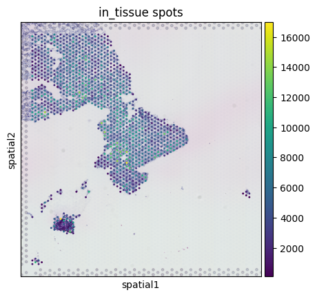
Visualizing the spots over a downscaled version of the WSI

# visualize the spots over a downscaled version of the full resolution image
save_dir = '.'
st.save_spatial_plot(save_dir)

/home/guillaumejaume/Documents/project_rosai/HEST/src/hest/HESTData.py:1570: FutureWarning: Use `squidpy.pl.spatial_scatter` instead.
  fig = sc.pl.spatial(adata, show=False, img_key="downscaled_fullres", color=[key], title=f"in_tissue spots", return_fig=True, **pl_kwargs)

Saving to pyramidal tiff and h5

Save HESTData object to .tiff + expression .h5ad and a metadata file.

# Warning saving a large image to pyramidal tiff (>1GB) can be slow on a hard drive.
st.save(save_dir, pyramidal=True)

Tissue segmentation

We integrated 2 tissue segmentation methods:

• Image processing-based using Otsu thresholding

• Deep learning-based using a fine-tuned DeepLabV3 ResNet50

save_dir = '.'

name = 'tissue_seg_otsu'
st.segment_tissue(method='otsu') 
st.save_tissue_seg_pkl(save_dir, name)

name = 'tissue_seg_deep'
st.segment_tissue(method='deep') 

/tmp/ipykernel_3742544/352998490.py:5: DeprecationWarning: Call to deprecated function save_tissue_seg_pkl.
  st.save_tissue_seg_pkl(save_dir, name)

	tissue_id	geometry
0	0	POLYGON ((4412 14007, 4402 14017, 4412 14027, ...
1	1	POLYGON ((2156.071 1865.929, 2156.063 1865.923...

Changing the Patching/pooling size

Patching

You can change the size of patches around the spots with dump_patches:

# directory where the patch .h5 will be saved
patch_save_dir = './processed'
new_patch_size = 224

st.dump_patches(
    patch_save_dir,
    name='demo',
    target_patch_size=new_patch_size,
    target_pixel_size=0.5 # pixel size of the patches in um/px after rescaling
)

Changing the Pooling size

You can change the pooling size of Xenium/Visium HD samples stored in HESTData.adata with the following:

from hest.readers import pool_transcripts_xenium
from hest import iter_hest

new_spot_size = 200
new_patch_size = 224
patch_save_dir = './processed'

# Iterate through a subset of hest
for st in iter_hest('../hest_data', id_list=['TENX95'], load_transcripts=True,):
    print(st.transcript_df)

    st.adata = pool_transcripts_xenium(
                    st.transcript_df, # Feel free to convert st.transcript_df to a Dask DataFrame if you are working with limited RAM.
                    st.pixel_size, 
                    key_x='he_x',
                    key_y='he_y',
                    spot_size_um=new_spot_size
                )

    # We change the spots, so we need to re-extract the patches
    st.dump_patches(
        patch_save_dir,
        name='demo',
        target_patch_size=new_patch_size, # target patch size in 224
        target_pixel_size=0.5 # pixel size of the patches in um/px after rescaling
    )

Batch effect visualization

import pandas as pd
from hest.batch_effect import filter_hest_stromal_housekeeping, get_silhouette_score, plot_umap

meta_df = pd.read_csv('../assets/HEST_v1_3_0.csv')


meta_df = meta_df[
    (meta_df['st_technology'] == 'Visium') & 
    (meta_df['disease_state'] == 'Cancer') & 
    (meta_df['oncotree_code'] == 'IDC') & 
    (meta_df['species'] == 'Homo sapiens')
]

# We filter spots, such that:
# - we only keep the most stable housekeeping genes (based on https://housekeeping.unicamp.br/?download)
# - we only keep the spots under the stroma (based on CellViT segmentation)
adata_list = filter_hest_stromal_housekeeping(meta_df, hest_dir='../hest_data')

labels = meta_df['id'].values
score = get_silhouette_score(adata_list, labels=labels)
# (-1: strong overlap between clusters, can be indicative of a small batch effect, 1: poor overlap between clusters, can be indicative of a strong batch effect)
print(f'Silhouette score is {score}')


plot_umap(adata_list, labels, 'batch_whole_tissue.png', umap_kwargs={'min_dist': 0.6})

Loading transcripts (for Xenium only)

The transcript dataframe contains the following columns:

• cell_id (default Xenium Explorer flag): id of cell containing this transcript

• he_x, he_y: x, y coordinate or transcript on the HE WSI in pixels (aligned with a non-rigid transformation)

• feature_name: name of transcript

• qv (default Xenium Explorer flag): Phred-scaled quality value (Q-Score) estimating the probability of incorrect call

from hest import iter_hest

# Iterate through a subset of hest
for st in iter_hest('../hest_data', id_list=['TENX105'], load_transcripts=True):
    print(st.transcript_df)

Warning: The segmentation contained in ‘xenium_seg/’ (accessed with st.get_shapes(‘xenium_cell’, ‘he’) or st.get_shapes(‘xenium_nucleus’, ‘he’)) is different than the CellViT segmentation. It was obtained by the Xenium instrument directly by segmenting the DAPI stained image, the DAPI segmented cells were then aligned to H&E with a non rigid transform.

Linking transcripts with cells

Each transcript is associated with a cell id (derived by the Xenium analyzer directly). See column cell_id in the transcript dataframe.

transcripts = st.transcript_df
shapes = st.get_shapes('xenium_cell', 'he').shapes

cell_id = 1

# Print the transcripts associated with a particular cell
print(transcripts[transcripts['cell_id'] == cell_id])
print(shapes[shapes.index == cell_id])